Fuzzy Clustering
Note: This post was originally published on my old blog on 2018-05-01 and has been transferred here. I have rewritten parts of the original article for clarity and style while keeping the main story and facts intact. Where my current self disagreed with or wanted to expand on the original, I added margin notes signed — Eke, May 2026.
I first ran into fuzzy clustering during a machine learning course in my undergrad. The idea that a single data point could belong to multiple clusters at once felt wrong ◆ Eight years later, this still makes me smile. The friction I felt then is exactly what makes fuzzy clustering interesting. If the answer were obvious, you would not need an algorithm. What I did not appreciate at the time was how naturally this maps onto Bayesian thinking: the membership coefficients are essentially posterior probabilities over cluster assignments. — EKE, May 2026 . Either something is in a group or it is not, right?
Turns out, the world is rarely that clean.
Think about a customer who buys both hiking gear and cooking equipment. Do you put them in the "outdoors" segment or the "food" segment? A hard clustering algorithm forces you to pick one. Fuzzy clustering says: they are 60% outdoors, 40% food. That is more useful for most real problems ◆ Customer segmentation was the go-to example in every 2018 ML tutorial, and I was no exception. The example is fine but it hides a subtle point: the membership coefficients are only as good as the feature space they live in. If your features do not separate the underlying behaviors, the coefficients will look uniform and tell you nothing. I have seen plenty of projects where fuzzy clustering gave near-uniform 1/C membership across all points, and the team concluded the algorithm did not work. The algorithm was fine. The features were the problem. — EKE, May 2026 .
This post walks through what fuzzy clustering is, how the Fuzzy C-Means algorithm works under the hood, and how to implement it in R and Python.
Clustering in two flavours
Cluster analysis is the task of grouping objects so that objects in the same group are more similar to each other than to objects in other groups1. There are dozens of algorithms, but they fall into two broad categories:
- Hard clustering: every point belongs to exactly one cluster. K-means, hierarchical clustering, DBSCAN all work this way.
- Soft (fuzzy) clustering: every point has a membership coefficient for each cluster, ranging from 0 to 1. The coefficients sum to 1 across clusters.
Hard clustering is simpler and faster. Fuzzy clustering is more expressive ◆ This hard/soft binary is itself a simplification. DBSCAN has noise points that belong to no cluster, hierarchical clustering has merges that are fuzzy until you cut the dendrogram, and spectral clustering operates in an embedding where distances themselves are soft. The lines are blurrier than I made them sound here. If I were writing this today I would frame it as a spectrum of assignment granularity rather than a hard dichotomy. — EKE, May 2026 . Which one you use depends on whether your data has clear boundaries or graded transitions.
Fuzzy C-Means
The Fuzzy C-Means (FCM) algorithm, developed by Dunn in 1973 and improved by Bezdek in 19812, is the fuzzy counterpart to K-means. The core idea is the same: find cluster centers and assign points to them. But instead of a hard assignment, each point gets a membership value for every cluster.
The objective function
FCM minimizes the following:
$$ J_m = \sum_{i=1}^{N} \sum_{j=1}^{C} u_{ij}^m |x_i - c_j|^2 $$
where:
- $N$ is the number of data points
- $C$ is the number of clusters
- $u_{ij}$ is the membership of point $i$ in cluster $j$
- $m$ is the fuzziness parameter ($m > 1$), controlling how soft the boundaries are
- $x_i$ is the $i$-th data point
- $c_j$ is the center of cluster $j$
Higher $m$ means fuzzier clusters. Standard practice uses $m = 2$3 ◆ One thing I glossed over completely: the choice of $m$ is not arbitrary, and $m = 2$ is not always optimal. Small $m$ (close to 1) makes FCM behave like K-means with near-binary assignments. Large $m$ (above 3) flattens memberships toward uniformity and can make clusters indistinguishable. There is literature on optimizing $m$ via cluster validity indices, but in practice most people pick 2 because Bezdek said so. I have seen datasets where $m = 1.5$ gave much cleaner separation, and others where $m = 3$ was needed to avoid degenerate solutions. Experiment. — EKE, May 2026 .
The algorithm
FCM iterates between two updates until convergence:
1. Update membership coefficients:
$$ u_{ij} = \frac{1}{\sum_{k=1}^{C} \left( \frac{|x_i - c_j|}{|x_i - c_k|} \right)^{\frac{2}{m-1}}} $$
This says: if a point is close to cluster $j$ relative to other clusters, its membership in $j$ will be high.
2. Update cluster centers:
$$ c_j = \frac{\sum_{i=1}^{N} u_{ij}^m x_i}{\sum_{i=1}^{N} u_{ij}^m} $$
Each cluster center is a weighted average of all points, weighted by their membership to that cluster.
The algorithm repeats these steps until the objective function stops changing (or changes less than some tolerance)4
◆
A real issue I did not mention: local minima. FCM, like K-means, is sensitive to initialization. Different random starts can produce different clusterings, especially with higher $m$ or many clusters. The standard fix is to run the algorithm multiple times with different seeds and keep the run with the lowest $J_m$, but that adds computation. The skfuzzy implementation does not do this automatically, and fanny() in R has limited support for it. If reproducibility matters, set a seed and report it. — EKE, May 2026
.
K-means is a special case of FCM. If you set $m \to 1$, the memberships become binary and FCM collapses into K-means. In practice, FCM with $m = 2$ is the standard choice.
What the output looks like
After convergence, each point has a vector of $C$ membership values. A point near the core of a cluster might have membership $[0.95, 0.03, 0.02]$. A point on the boundary between two clusters might have $[0.45, 0.50, 0.05]$ ◆ I used to treat these vectors as pure assignment probabilities. They are not. The membership $u_{ij}$ depends on the position of all cluster centers, not just the distance to cluster $j$. If cluster centers shift because of a faraway group, the membership of a point that has not moved can change. This makes temporal or cross-dataset comparisons of membership values tricky unless the cluster centers are aligned first. — EKE, May 2026 .
When would you use fuzzy over hard clustering?
Fuzzy clustering shines when cluster boundaries are not sharp. Examples include image segmentation (a pixel can be part sky and part tree), customer segmentation (people have mixed interests), and biological data where expression states grade into each other. Use hard clustering when you need categorical assignments or when your data has natural, well-separated groups.
Fuzzy C-Means in R
The cluster package has fanny() for fuzzy clustering
◆
fanny() is fine for basic use, but it has limitations. It cannot handle large datasets well (the distance matrix grows quadratically), and it does not expose the fuzziness parameter $m$ directly (it uses a different parametrisation called memb.exp). The ppclust and fcclust packages offer more modern FCM implementations with better initialization options, but fanny() remains the most battle-tested. If I were writing this section today, I would also mention the clustMixType package for mixed-type data, which is a common real-world scenario. — EKE, May 2026
. Let us run it on the Iris dataset.
library(cluster)
library(factoextra)
library(tidyverse)

iris_df <- iris %>%
  mutate(spec_idx = row_number()) %>%
  unite("species", Species, spec_idx, sep = "-", remove = TRUE) %>%
  column_to_rownames("species") %>%
  select(-species)

res.fanny <- fanny(iris_df, 3)

head(res.fanny$membership, 7)Output:
[,1]       [,2]       [,3]
setosa-1  0.9115847 0.03714162 0.05127368
setosa-2  0.8641378 0.05659841 0.07926381
setosa-3  0.8720433 0.05381542 0.07414133
setosa-4  0.8459146 0.06419306 0.08989232
setosa-5  0.9001651 0.04205859 0.05777633
setosa-6  0.7648869 0.09848692 0.13662620
setosa-7  0.8601062 0.05878600 0.08110779
The setosa points all have memberships above 0.76 in cluster 1. Clear assignment. The versicolor and virginica points will show more spread ◆ A detail I skipped: look at setosa-6. Its membership in cluster 1 is 0.76, noticeably lower than the others. This is a real effect, not noise. Some individual Iris plants in the Fisher dataset have petal/sepal measurements that push them toward the versicolor boundary. If I were using these memberships downstream, I would flag setosa-6 as a borderline case worth inspecting. Membership coefficients are diagnostic tools, not just output. — EKE, May 2026 .
fviz_cluster(res.fanny, ellipse.type = "convex",
             palette = c("#00AFBB", "#E7B800", "#FC4E07"),
             ggtheme = theme_minimal(), legend = "right")
Figure 1. Fuzzy cluster plot for the Iris dataset.
Setosa forms a tight cluster on the left. Versicolor and virginica overlap in the middle. That overlap is exactly what the membership coefficients capture. The silhouette plot tells a similar story:
fviz_silhouette(res.fanny, palette = c("#00AFBB", "#E7B800", "#FC4E07"),
                ggtheme = theme_minimal())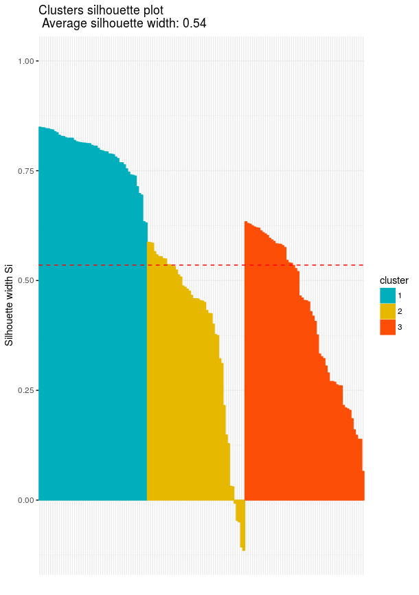
Figure 2. Silhouette plot for the fuzzy clustering result.
The average silhouette width of 0.42 is decent. Most points fit their assigned clusters reasonably well, but the overlap between versicolor and virginica pulls the average down.
Fuzzy C-Means in Python
Python does not have FCM in scikit-learn
◆
In 2026 this is still true. scikit-learn has never added fuzzy clustering to its core API. The maintainers have discussed it multiple times on GitHub issues and always punted, mainly because the demand is low relative to maintenance cost. scikit-fuzzy has been the defacto standard since, but it has not seen a major release in years. If you need something production-ready with modern Python support, consider fuzzy-c-means (PyPI) or implementing the update equations yourself in 30 lines of numpy. The algorithm is simple enough that a custom implementation is often cleaner than wrangling an unmaintained dependency. — EKE, May 2026
. The scikit-fuzzy (skfuzzy) library fills the gap5. Let us generate synthetic data with three known clusters and see how FCM recovers them.
import numpy as np
import skfuzzy as fuzz
import matplotlib.pyplot as plt
import seaborn as sns

sns.set_style("white")
np.random.seed(42)

centers = [[1, 3], [2, 2], [3, 8]]
sigmas  = [[0.3, 0.5], [0.5, 0.3], [0.5, 0.3]]

xpts, ypts = np.array([]), np.array([])
for (xmu, ymu), (xsigma, ysigma) in zip(centers, sigmas):
    xpts = np.append(xpts, np.random.normal(xmu, xsigma, 200))
    ypts = np.append(ypts, np.random.normal(ymu, ysigma, 200))

plt.figure(figsize=(8, 6))
plt.scatter(xpts, ypts, c=["b"]*200 + ["orange"]*200 + ["g"]*200, s=10)
plt.title("Test data: 600 points, 3 clusters")
plt.show()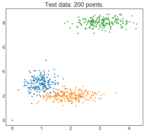
Figure 3. Synthetic test data with three visible clusters.
Three visible clusters. The question is how many clusters FCM finds on its own. The Fuzzy Partition Coefficient (FPC) tells us. FPC ranges from 0 to 1, with 1 meaning perfectly separated clusters ◆ FPC and its close relative the Normalized Fuzzy Partition Coefficient (NFPC) are useful heuristics, but they have a well-known bias: they favour compact, spherical clusters with similar sizes. If your data has elongated clusters, varying densities, or very different sizes, FPC will mislead you. There are alternatives: the Xie-Beni index, the Fukuyama-Sugeno index, and the silhouette width (which works for fuzzy assignments too). I did not know about these in 2018 and relied on FPC alone. Do not make the same mistake. — EKE, May 2026 . Let us fit models with 2 through 10 clusters and compare.
alldata = np.vstack((xpts, ypts))
fpcs = []

fig, axes = plt.subplots(3, 3, figsize=(10, 10))
colors = ["b", "orange", "g", "r", "c", "m", "y", "k", "Brown"]

for ncenters, ax in enumerate(axes.ravel(), start=2):
    cntr, u, _, _, _, _, fpc = fuzz.cluster.cmeans(
        alldata, ncenters, 2, error=0.005, maxiter=1000, init=None
    )
    fpcs.append(fpc)

    cluster_membership = np.argmax(u, axis=0)
    for j in range(ncenters):
        ax.scatter(xpts[cluster_membership == j],
                   ypts[cluster_membership == j],
                   c=colors[j], s=8)
    ax.scatter(cntr[:, 0], cntr[:, 1], marker="s", c="red", s=60)
    ax.set_title(f"Centers = {ncenters}, FPC = {fpc:.2f}")
    ax.axis("off")

plt.tight_layout()
plt.show()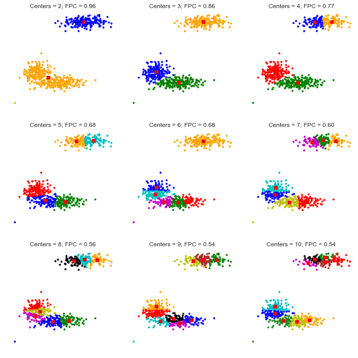
Figure 4. Cluster comparison across different numbers of centers with FPC values.
The FPC peaks at 2 clusters, not 3. That is unexpected. Let us check the FPC values directly:
plt.figure(figsize=(8, 5))
plt.plot(range(2, 11), fpcs, "o-", color="#731810")
plt.xlabel("Number of clusters")
plt.ylabel("Fuzzy Partition Coefficient")
plt.title("FPC vs Number of Clusters")
plt.show()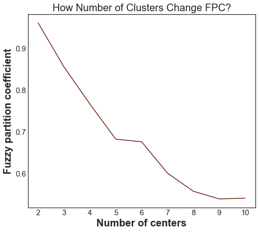
Figure 5. Fuzzy Partition Coefficient as a function of cluster count.
FPC peaks at 2 clusters (0.82) and drops steadily after that. Why would a dataset with three real clusters have a higher FPC at 2?
Look at the data again. The two left clusters (centers at [1,3] and [2,2]) are close together. FCM with 2 clusters merges them into one and keeps the right cluster separate. The resulting partition is cleaner in the FPC sense because the merged cluster is still compact. FPC penalises overlap, and the two left clusters overlap significantly.
FPC is not the ground truth. It tells you how clean your partition is, not whether it matches reality. Always pair FPC with domain knowledge and visual inspection. If you know your data has three meaningful groups, three clusters is the right answer regardless of what FPC says.
Closing thoughts
Fuzzy clustering is not a replacement for hard clustering. It is a different tool for a different kind of problem. Use it when your data has graded boundaries, when a point can reasonably belong to multiple groups, or when you need probabilities instead of labels ◆ If I were writing this post today, I would add a third use case: diagnostic tool. The membership distribution across points can tell you things about your data that hard assignments hide. High-entropy membership vectors (where no cluster gets above 0.5) are a strong signal that your data does not cluster well, your feature space is poorly chosen, or the number of clusters is wrong. A hard clustering algorithm will still assign every point to some cluster and give you confident-looking labels. Fuzzy clustering forces the ambiguity into the open. That alone is worth the price of entry. — EKE, May 2026 .
The FCM algorithm itself is simple, well-studied, and implemented in both R and Python6. Start with $m = 2$, validate with FPC and visual inspection, and treat the membership coefficients as the rich information they are ◆ If there is one thing I want readers to take away from this 2026 annotation, it is this: the membership coefficients are not the final answer. They are the beginning of the analysis. Plot their distributions. Check for high-entropy points. Compare them across runs with different random seeds. Cluster the membership vectors themselves to see if there are meta-clusters of points with similar assignment profiles. The membership matrix often contains structure that is invisible in the original feature space. I missed all of this in 2018. I hope you do not. — EKE, May 2026 .
-
The classic definition from Kaufman and Rousseeuw (1990), Finding Groups in Data. ↩
-
Dunn's 1973 paper introduced the fuzzy ISODATA algorithm; Bezdek generalised it into FCM in 1981. ↩
-
Schwammle, V. & Jensen, O.N. (2010). A simple and fast method to determine the parameters for fuzzy c-means cluster analysis. Bioinformatics, 26(22), 2841-2848. doi:10.1093/bioinformatics/btq534. They propose a method to choose $m$ and $C$ simultaneously by finding the point where clustering on randomised data no longer detects structure. ↩
-
Matteucci, M. A Tutorial on Clustering Algorithms - Fuzzy C-Means. Available at matteucci.faculty.polimi.it. A clear, visual walkthrough of the FCM algorithm with interactive demos. ↩
-
Scikit-Fuzzy documentation. Fuzzy c-means clustering. Available at pythonhosted.org/scikit-fuzzy. The official example gallery for the skfuzzy library. ↩
-
Doring, C., Lesot, M.-J. & Kruse, R. (2006). Data analysis with fuzzy clustering methods. Computational Statistics & Data Analysis, 51(1), 192-214. doi:10.1016/j.csda.2006.04.030. A comprehensive survey of the fuzzy clustering landscape, covering objective function methods, ACE, and FMLE. ↩